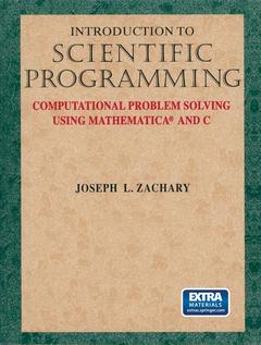
Introduction to Scientific Programming, 1998 Computational Problem Solving Using Mathematica® and C

Developed over a period of two years at the University of Utah Department of Computer Science, this course has been designed to encourage the integration of computation into the science and engineering curricula. Intended as an introductory course in computing expressly for science and engineering students, the course was created to satisfy the standard programming requirement, while preparing students to immediately exploit the broad power of modern computing in their science and engineering courses.

1 Computational Science.- 1.1 Experiment, Theory, and Computation.- 1.2 Solving Computational Problems.- 1.3 Onward.- 2 Population Density: Computational Properties of Numbers.- 2.1 Model.- 2.2 Method.- 2.3 Implementation.- 2.4 Arithmetic Expressions.- 2.5 Rational Numbers.- 2.6 Rational Numbers in Mathematica.- 2.7 Floating-Point Numbers.- 2.8 Floating-Point Numbers in Mathematica.- 2.9 Assessment.- 2.10 Key Concepts.- 2.11 Exercises.- 3 Eratosthenes: Significant Digits and Interval Arithmetic.- 3.1 Model.- 3.2 Method.- 3.3 Implementation.- 3.4 Implementation Assessment.- 3.5 Method Assessment.- 3.6 Model Assessment.- 3.7 Problem Assessment.- 3.8 Key Concepts.- 3.9 Exercises.- 4 Stairway to Heaven: Accumulation of Roundoff error.- 4.1 An Inductive Model.- 4.2 Summing the Harmonic Series.- 4.3 Accumulation of Roundoff Error.- 4.4 Assessment.- 4.5 Key Concepts.- 4.6 Exercises.- 5 Kitty Hawk: Programmer-Defined Functions.- 5.1 Model.- 5.2 Method.- 5.3 Implementation.- 5.4 Assessment.- 5.5 Key Concepts.- 5.6 Exercises.- 6 Baby Boom: Symbolic Computation.- 6.1 Simple Interest.- 6.2 Compound Interest.- 6.3 Continuous Interest.- 6.4 Assessment.- 6.5 Key Concepts.- 6.6 Exercises.- 7 Ballistic Trajectories: Scientific Visualization.- 7.1 Ballistic Motion.- 7.2 Scientific Visualization.- 7.3 Motion Functions.- 7.4 Two-Dimensional Plots.- 7.5 Lists.- 7.6 Multiple-Curve Plots.- 7.7 Parametric Plots.- 7.8 Animation.- 7.9 Key Concepts.- 7.10 Exercises.- 8 The Battle for Leyte Gulf: Symbolic Mathematics.- 8.1 Fixed Trajectory.- 8.2 Arbitrary Trajectories.- 8.3 Effects of Drag.- 8.4 Piecewise Trajectories.- 8.5 Final Assessment.- 8.6 Key Concepts.- 8.7 Exercises.- 9 Old Macdonald’s Cow: Imperative Programming.- 9.1 Solving Equations in Mathematica.- 9.2 Bisection Method.- 9.3 A Bisection Function.- 9.4 Assessment.- 9.5 Key Concepts.- 9.6 Exercises.- 10 Introduction to C.- 10.1 Mathematica Background.- 10.2 C Background.- 10.3 An Example C Program.- 10.4 Interpreters versus Compilers.- 10.5 Differences Between Mathematica and C.- 10.6 Learning C.- 10.7 Eratosthenes’s Problem.- 10.8 Kitty Hawk Problem.- 10.9 Key Concepts.- 10.10 Exercises.- 11 Robotic Weightlifting: Straight-Line Programs.- 11.1 Trigonometry of a Link Diagram.- 11.2 Components of a Straight-Line Program.- 11.3 Types.- 11.4 Expressions.- 11.5 Simple Statements.- 11.6 Main Function.- 11.7 Libraries.- 11.8 Assessment.- 11.9 Key Concepts.- 11.10 Exercises.- 12 Sliding Blocks: Conditionals and Functions.- 12.1 An Infinite Ramp without Friction.- 12.2 An Infinite Ramp with Friction.- 12.3 A Finite Ramp with Friction.- 12.4 Programmer-Defined Functions.- 12.5 Assessment.- 12.6 Key Concepts.- 12.7 Exercises.- 13 Rod Stacking: Designing with Functions.- 13.1 Decomposing the Problem.- 13.2 Design.- 13.3 Implementation.- 13.4 Assessment.- 13.5 Key Concepts.- 13.6 Exercises.- 14 Newton’s Beam: Repetition.- 14.1 Newton’s Method.- 14.2 Implementation of Newton’s Method.- 14.3 Bisection Method Implementation.- 14.4 Assessment.- 14.5 Key Concepts.- 14.6 Exercises.- 15 Corrugated Sheets: Multiple-File Programs.- 15.1 Numerical Integration.- 15.2 Rectangular Method.- 15.3 Rectangular Method Implementation.- 15.4 Trapezoidal Method.- 15.5 Trapezoidal Method Implementation.- 15.6 Multiple-File Programs.- 15.7 Comparison of Rectangular and Trapezoidal Methods.- 15.8 Key Concepts.- 15.9 Exercises.- 16 Harmonic Oscillation: Structures and Abstract Datatypes.- 16.1 Newton’s Method with Complex Roots.- 16.2 Rod Stacking Revisited.- 16.3 Newton’s Method Revisited.- 16.4 Assessment.- 16.5 Key Concepts.- 16.6 Exercises.- 17 Heat Transfer in a Rod: Arrays.- 17.1 Modeling Heat Flow.- 17.2 A Finite-Element Method.- 17.3 Implementation.- 17.4 Assessment.- 17.5 Key Concepts.- 17.6 Exercises.- 18 Visualizing Heat Transfer: Arrays as Parameters.- 18.1 Arrays as Parameters.- 18.2 File Input.- 18.3 File Output.- 18.4 Assessment.- 18.5 Key Concepts.- 18.6 Exercises.- A Mathematica Capabilities.- A.1 Units.- A.2 Typeset Mathematics.- A.3 Floating-Point Simulation.- A.4 Arbitrary-Precision Numbers.- C C Library Functions.- D.1 Floating-Point Syntax.- D.2 Typeset Mathematics.- D.3 Special Constants418 D.4 Symbolic Capabilities.